Price Models using Quantile Regression

Modelling the Bitcoin price with time is often done using Ordinary Least Squares (OLS) regression. Quantile Regression (QR) offer some unique advantages by showcasing not just where average prices are expected to center but also how broadly they might fluctuate.

As such, QR is particularly valuable for predicting the full spectrum of possible price movements and to understand the best and worst-case scenarios.

You will find both OLS and QR models in the Bitcoin Research Lab.

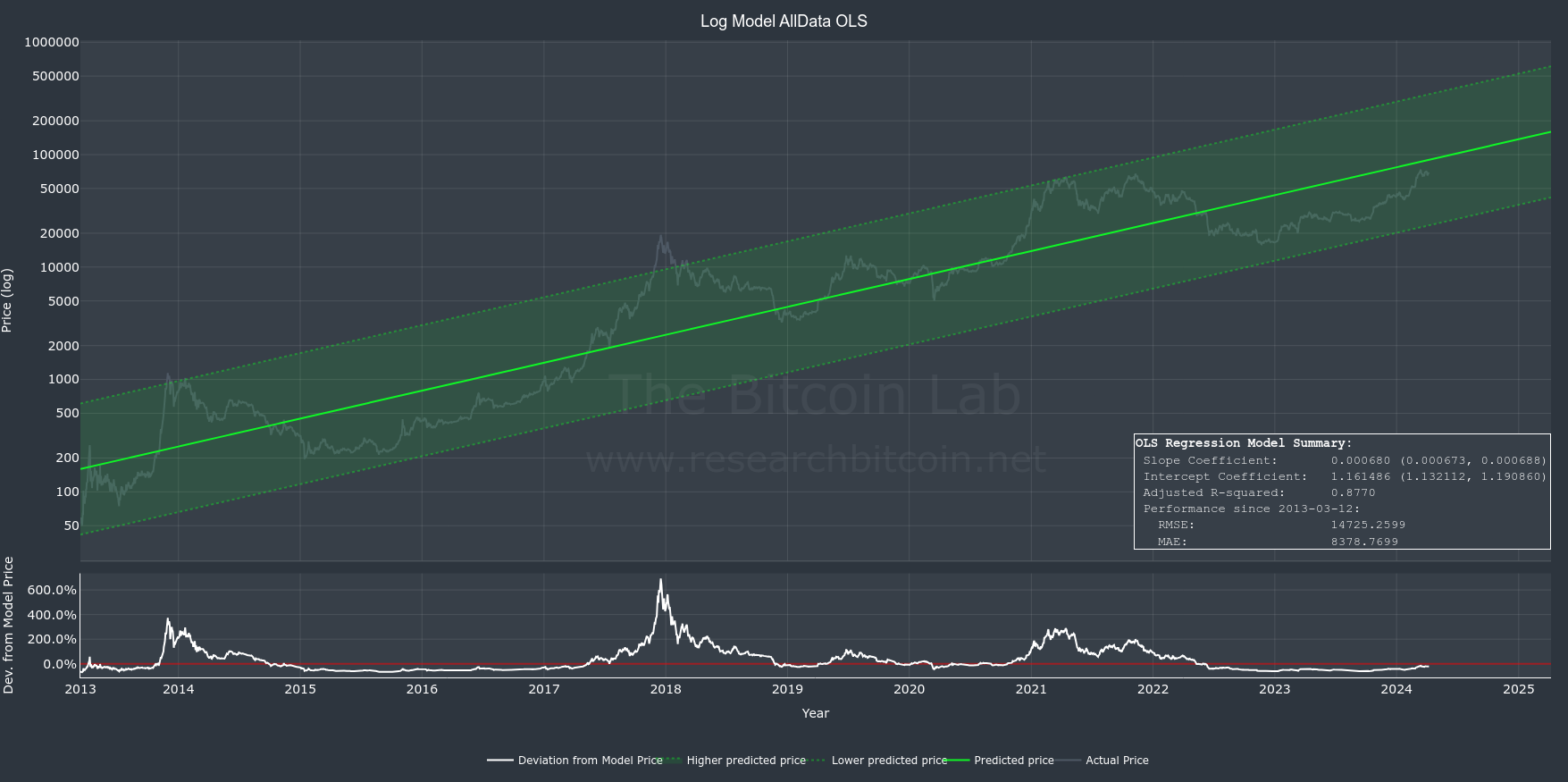
Ordinary Least Squares - OLS

Ordinary Least Squares (OLS) is the most commonly used statistical method used for linear regression analysis. It is a technique used to estimate the relationship between independent variable(s) (e.g. time) and a dependent variable (e.g. Bitcoin price).

OLS finds the best-fitting line that models the data by minimizing the sum of the squares of the differences between the observed and predicted values.

OLS is favored for its simplicity, interpretability, and efficiency, making it the first choice when the key assumptions are reasonably met. We will discuss the key assumptions in a minute.

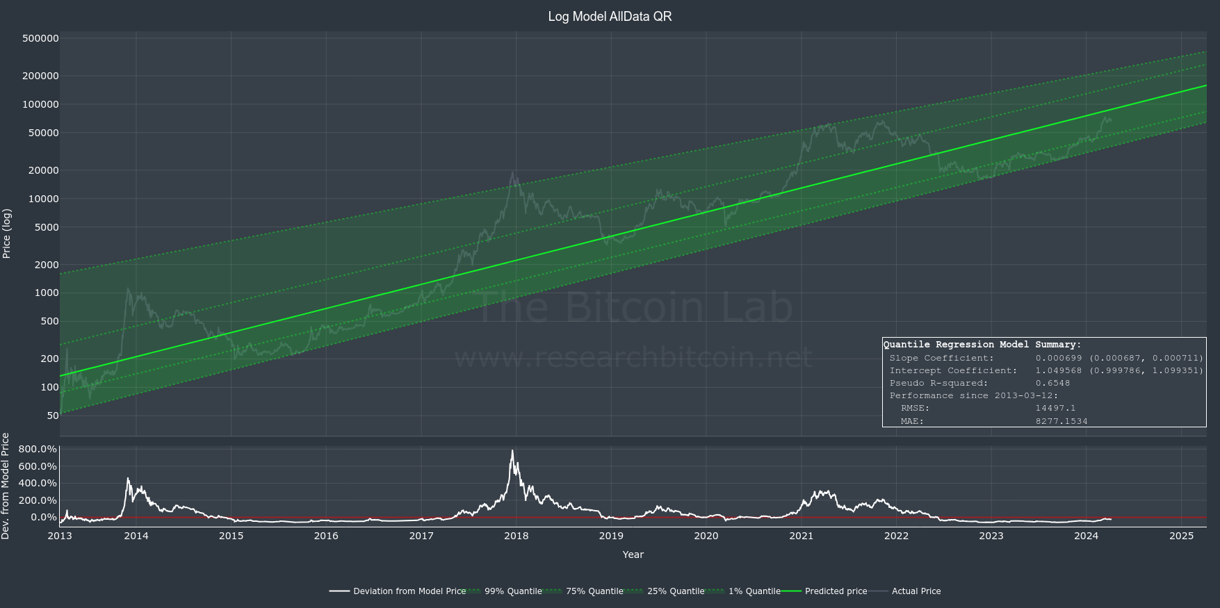
Quantile Regression - QR

Quantile Regression (QR) is a another statistical technique used for linear regression analysis. It can also be used to estimate the relationship between variable(s) (e.g. time) and a dependent variable (e.g. Bitcoin price).

QR estimates the conditional quantiles of a dependent variable's distribution (e.g. Bitcoin price), given the independent variables (e.g. time).

This approach allows for robust analysis even when datasets have asymmetrical distributions and outliers. QR has a higher tolerance for non-normality and heteroscedasticity than OLS models. We will discuss the key assumptions next.

Common assumptions for OLS and QR

OLS and QR share foundational assumptions critical for their effective application. These assumptions ensure the validity and reliability of the regression analysis:

• Independence: Observations are assumed to be independent across individuals, preventing data points from influencing each other's outcomes.
• No Perfect Multicollinearity: No independent variable is a perfect linear combination of any other variables, ensuring the stability of the model and the interpretability of the coefficients.
• Correct Model Specification: The relationships between dependent and independent variables must be correctly specified, including the correct functional form and inclusion of relevant variables.

Differences in key assumptions

While both OLS and QR share key assumptions, they diverge significantly in some underlying assumptions about the error distribution and variance:

• Error Distribution: OLS assumes that the error terms are normally distributed (especially for the purpose of hypothesis testing). QR, in contrast, does not require the error terms to follow a normal distribution, making it more adaptable to outliers and non-normal data.
• Homoscedasticity: OLS requires that the error terms have constant variance (homoscedasticity) across observations. QR is less restrictive, accommodating heteroscedasticity, which allows for variance in error terms across different quantiles of the dependent variable.
• Focus of Estimation: OLS estimates the mean of the dependent variable conditional on the independent variables. QR estimates various quantiles (e.g., median) of the dependent variable, providing a more detailed view of the distribution and its potential asymmetry.

Time-series and autocorrelation

In OLS and QR, time-series data provides a particular challenge known as autocorrelation. Autocorrelation means that past values can predict future ones, challenging the shared assumption of Independence (that each data point is independent).

For example, autocorrelation can lead to underestimation of the model's error terms. This can falsely increase the confidence in the model's predictions. Imagine forecasting Bitcoin prices; it might suggest a precision in prediction that isn't actually there, leading to overconfident investment decisions.

Specifically:

• Too Narrow Confidence Intervals (CI): Autocorrelation tends to reduce the estimated variance of the regression coefficients. This underestimation makes the confidence intervals narrower than they should be, suggesting a level of precision in the estimates that is not actually present.
• Inflated R-squared: The presence of autocorrelation can also inflate the R-squared value, which is a measure of the proportion of the variance in the dependent variable that is predictable from the independent variables. R-squared can appear misleadingly high because the model captures the serial correlation in the data rather than the actual relationship between the independent and dependent variables.

Practically, both OLS and QR should be investigated for the impact of autocorrelation and the need for method modifications evaluated. For OLS, techniques such as adding lagged variables or using robust standard errors might be employed. For QR, bootstrapping methods can help provide more accurate inference despite the presence of autocorrelation.

What are the Advantages of QR?

QR offers a valuable complement to OLS in modeling the Bitcoin price over time. OLS is the most effective, while QR is more robust in dealing with datasets characterized by non-normal distributions, heteroscedasticity and the presence of outliers (like Bitcoin price).

An important feature of QR is its ability to estimate the likely distribution of future prices at specific points in time. This contrasts sharply with OLS, which estimates an average price.

OLS provides an average price estimate along with a confidence interval CI that indicates the range within which the average price is likely to fall given a level of confidence. This approach primarily focuses on the central tendency of future prices.
On the other hand, QR delineates the future price distribution across various percentiles, such as the 1st and 99th, offering a comprehensive picture of the potential range of future prices, from lower to upper extremes.