Bitcoin Power Law Price Prediction Using Quantile Regression

The Bitcoin price can be modeled as a linear relationship between time and price in log-log space, meaning that both the time (x-axis) and the price (y-axis) are log transformed. A common statistical procedure to model linear relationship (in log-log space, and elsewhere) is to use Ordinary Least Squares regression (OLS).

An alternative statistical procedure is quantile regression (QR). While both OLS and QR can be used to predict the range of future prices, they do so from different statistical foundations.

OLS Prediction Intervals are meant to capture where a new data point will fall, considering both the error in estimating the mean and the inherent data variability.

Quantile Estimates (QR) provide more specific information about the distribution, focusing on extreme values and the overall shape of the distribution beyond just the central tendency.

Forecasting future prices

When the goal is to forecast future prices, QR has some potential advantages over OLS. Here are those I find most important:

• QR is more robust to outliers than OLS, which may be prudent given Bitcoin history of price "bubbles".
• QR allows modeling various quantiles of the price distribution, providing a more detailed analysis of potential outcomes at various probability levels (e.g. 5% and 95% quantiles). It therefore enables predictions that are more tailored to different risk scenarios, rather than just the central tendency.
• OLS assumes normal distribution of errors and symmetric distribution around the mean. QR does not.

Modelling the Bitcoin Price

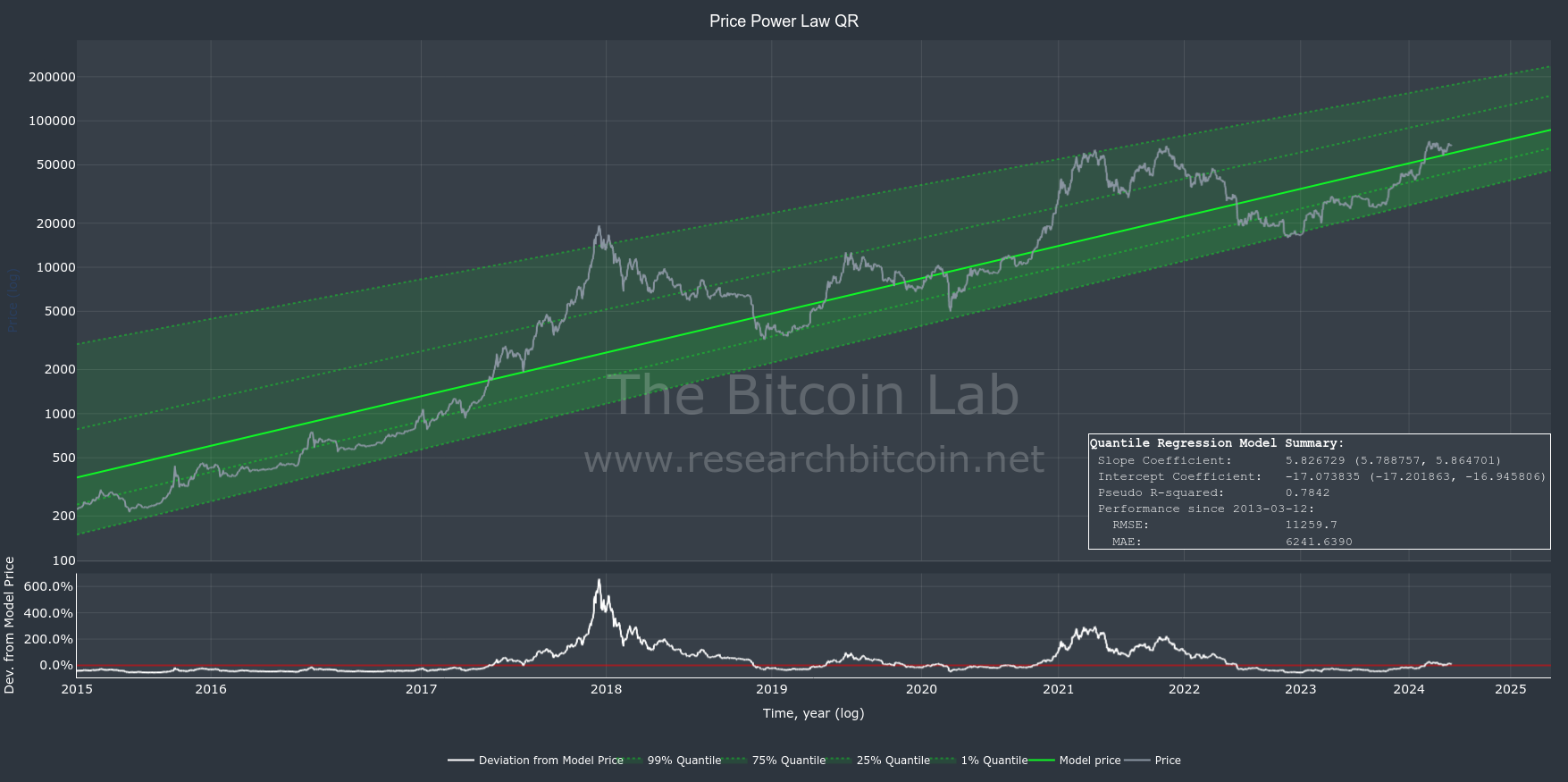
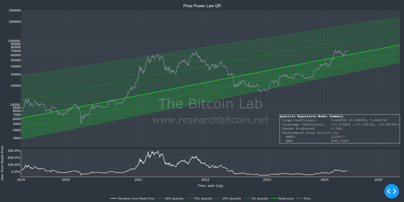
The Bitcoin Lab computes Power Law OLS and QR models that updates every day. As of today (2024-06-01), these are the current model specification:

Comparing the OLS and QR models

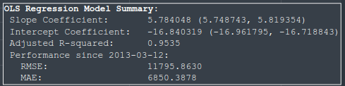
As evident from the model specification, the slope and intercept coefficients are quite similar, and share 95% confidence intervals.  The QR model has a slightly higher slope, and as such, is slightly more optimistic considering future prices.

A common metric to evaluate the fit of a model is the adjusted R-squared. The OLS model has a fit above 0.95 which is impressive indicating that it explain over 95% of the historic bitcoin price. Unfortunately, one cannot compute a comparable R-squared for QR models (there are various statistical approaches, but none is directly comparable). The pseudo-R-squared reported here is 0.784, which is actually very good in my experience.

To compare the QR and OLS model we can instead evaluate the Mean Absolute Error (MAE). MAE measures the average magnitude of the errors in a set of predictions, without considering their direction. The MAE is easy to interpret and provides a clear, direct measure that can be used to directly compare models. As evident from the model summaries above, the QR model shows substantially (almost 9%) lower MAE than the OLS model. A lower MAE is consistent with the QR model being most accurate.

At the very least, the QR model is not inferior to the OLS model.

Comparing price predictions

The QR model is particularly useful in forecasting price ranges. Computing the 5 and 95% quantiles effectively provides a predicted interval within which future prices are expected to lie with high probability.

For OLS it is also possible to construct prediction intervals around the model where future might lie. The nature of OLS is to estimate the central tendency around which future predictions are made (but assumes normal distribution of errors and symmetry around the mean).

If the goal is to understand or predict the extremes of price distribution, QR would be more directly applicable. The MAE indicates that the QR model is at least as accurate as the OLS model (based on historical data).  This is why I favor QR to forecast future prices.

Price Prediction for 2026-01-01

OLS:
The Lower Prediction Limit and the Upper Prediction Limit denote the prices which Bitcoin will not fall below and above, respectively, with 95% confidence.

Lower Prediction Limit: 29 570 USD
Higher Prediction Limit: 531 789 USD
Model price: 125 400 USD

Quantile Regression:

The Lower 5% Quantile and the Upper 95% Quantile represent the price which only 5% of prices to will fall below or above, respectively.

Lower 5% quantile: 65 895 USD
Model price (50% quantile): 106 333 USD
Upper 95% quantile: 284 536 USD

Conclusion

Using QR the price of Bitcoin should be within 65 895 and 284 536 on 2026-01-01.

Notice this range is considerably less narrow than the estimates provided by OLS. In all fairness, both OLS and QR models displays huge price intervals.

And please keep in mind, these are only models (which are certainly fun to play with, but I would not bet only based on on them).

A note on statistical assumptions

Both OLS and QR assume linearity, independent observation and not too highly correlated predictor variables. QR is less stringent in a couple of significant ways: Homoscedasticity is not assumed and normality of errors is not required. On the other hand, estimating the extreme quantiles (e.g. 1% and 99%) will inherently focus on the the tail and thus be more sensitive to outliers in those regions.

There are more rigorous tests that could and should be applied to both QR and OLS, e.g. bootstrapping. This assay is just a teaser for the interested.