Practical Implications of the Bitcoin Power Law Model

The Bitcoin Research Lab includes the Power Law Price model. This blog delves into the practical implications of the Power Law model. It contrasts the model's statistical robustness in logarithmic space against its applicability and relevance in the linear space that investors commonly navigate.

What is the Bitcoin Power Law Model

Mathematically, the Power Law Model is linear regression performed in log-log space. This means that prior to the linear regression analysis, both the time (x-axis) and the price (y-axis) are transformed into log space (log10). The log10 transformed value of 100 is 2, 1000 is 3, 1000 is 4...and so forth.

Many real-world phenomena exhibit exponential growth or decay which are not linear, but these may show linear characteristics after log transformation. The Power Law Model states that there is a linear relation between the log transformed time and log transformed price.

Many previous attempts to model the bitcoin price as a function of time have also used log transformed price. What sets the Power Model apart is the log transformation of time.

Technically, you cannot log transform 'a date', which therefore needs to be converted to a numeric metric. In the Power Law model, the time is defined as number of days since the Bitcoin genesis block (2009-01-03) starting at time = 1. The following date (2009-01-04) is time = 2..etc. This approach may appear arbitrary to some and logical to some. I will not discuss this further, suffice to say, I am not very critical to this approach but it do merit critical discussion.

Power Law Model specification

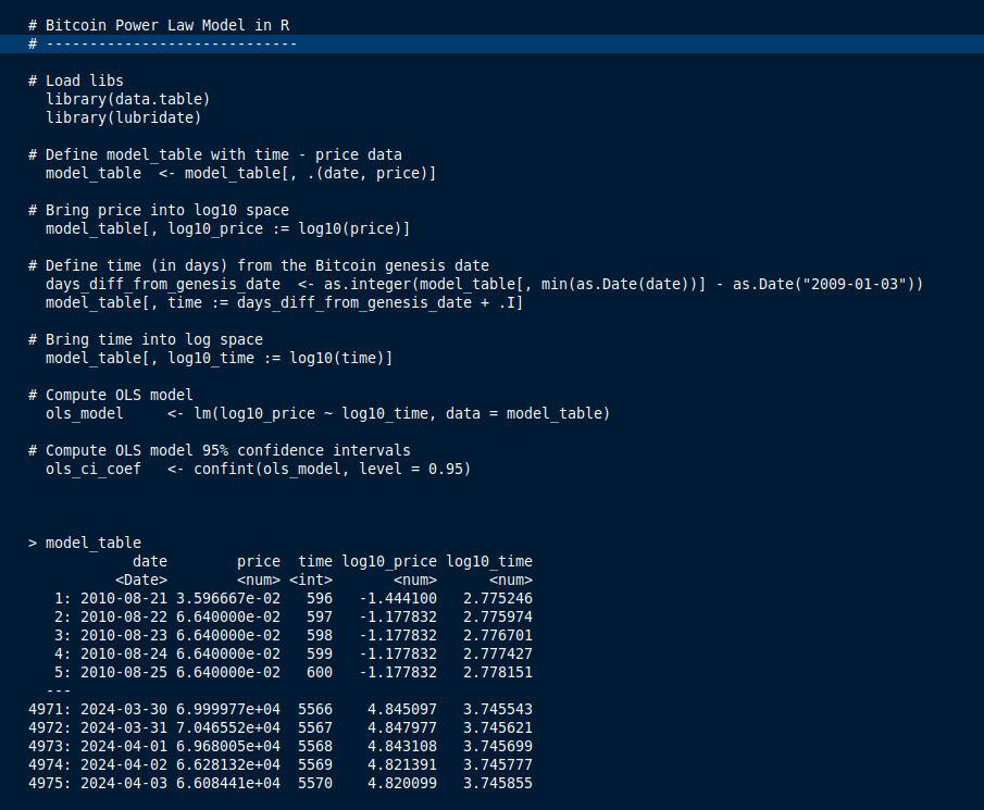
We have now established that the Bitcoin Power Law is linear regression analysis performed on log transformed time and price data. At the end of this blog post, I will provide the R code necessary for conducting this analysis.

Using all available price data from 2010-08-22 (earliest data I have) until today 2024-04-02, the linear regression analysis yields:

Price(t) = α + t^β
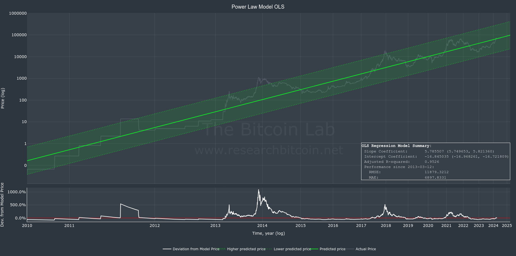
Slope Coefficient (α) = 5.7855             (95% CI 5.7497 to 5.8214)
Intercept Coefficient (β) = -16.8450    (95% CI -16.9683 to -16.7218)

So, what does the model predict the price to be today?
This can easily be computed by inserting the time (t) into the formula Price(t) = α + t^β.
Today (2024-04-03), 5570 days has elapsed since the genesis block. Derived from the Power Law formula above one Bitcoin should cost 67,156 US dollars. Impressively,this forecast aligns closely with the current price, which stands at 66,084 US dollars.

Model uncertainty and limitations

In the interest of scientific rigor, it is incumbent upon us to delineate the limitations of our model comprehensively, including an explicit discussion of its inherent uncertainties.

Slope Coefficient 95% CI =  5.7497 to 5.8214
Intercept Coefficient 95% CI  = -16.9683 to -16.7218
Adjusted R-squared: 0.9526

At first glance, the model specification is highly satisfactory. The 95% confidence intervals (CI) for the coefficients exhibit relatively narrow ranges. Additionally, the power model demonstrates a robust alignment to observed data. The R-squared value > 0.95 suggests that 95% of the variance in the dependent variable (price) can be accounted for by the independent variable (time).

But be aware! These model specifications are relevant within the context of log-log transformed analysis. It is crucial to understand that the interpretation of both coefficients and  the interpretation of R-square applies within the context of the log-transformed variables, and direct implications in linear space is not intuitive and requires careful consideration. In other words, even minor variations in the slope or intercept coefficients can lead to significant alterations in the price predictions.

One straightforward approach to elucidate the inherent uncertainties surrounding the Bitcoin Power Law price predictions in linear (normal) space involves the computation of the price alongside its 95% confidence interval. Fortunately, computing such intervals is a readily achievable with statistical software.

As delineated above, the central estimate for the predicted price is 67,156 US dollars. However, 95% confidence interval is much wider extending from a lower bound of 15,687 to an upper bound of 286,897 US dollars.

Examination of historical performance reveals that in 2013, Bitcoin's trading price exceeded the model's prediction by more than 900%. Similarly, at the peak of 2017, its trading price was 300% higher than the model's forecast price. In both instances, the observed prices surpassed the upper limit of the 95% confidence interval delineated by our model (which encompasses all data up to the present).

It is useful and interesting to compare the performance against other models in linear space. Relative to price logarithmic models, the Power Law Model exhibits enhanced predictive accuracy, as evidenced by its lower Root Mean Square Error (RMSE) and Mean Absolute Error (MAE) values—11880 versus 14722 for RMSE, and 6899 versus 8370 for MAE, respectively. In other terms, the Power Law model outperforms logarithmic models by approximately 21-23% in predictive accuracy.  Comprehensive data for these metrics, along with additional comparisons between models, can be found through the charts available at researchbitcoin.net/charts/.

How should we evaluate the power model?

The Power Law Model is likely the most accurate model of bitcoin price. In log space, the model's parameters exhibit both narrow ranges and robust characteristics, underscoring their internal validity. No doubt!

However, it is crucial to understand that failing to translate model specifications, like confidence intervals and R-squared values, into linear (normal) space detracts from its practical utility. Appreciating this perspective is crucial for rendering the data meaningful in real-world applications.

This discussion is primarily concerned with the model's utility in linear space—the perspective most relevant to investors. For investors, the Power Law Model is certainly interesting. Based on your investment strategy, you might contemplate incorporating this approach into your overall investing plan. However, the considerable breadth of its predicted price range somewhat constrains its utility for precise future price forecasts. This observation isn't so much a critique of the model as it is a caveat regarding its use. The larger range is a demonstration of the volatility of Bitcoin price which does not fit in any linear relationship.

Imagine you were back at the 2017/18 peak, when Bitcoin reach almost 20000 US dollars. An analysis of the Power Law model at that time would have indicated a have projected a price range for April 2024 spanning from 13,277 to 393,882 US dollars. Many investors, myself among them, might question the significance of this information in shaping an investment strategy.

And finally, the Power Law is a model derived from historical data. Just like all other models, there is no guarantee that it will be valid in the future. It may even fail completely.

R code for Power Law Model